Team Members: Felipe Godoy, Andrew Gauker, Amy Pollmann, Hetu Patel, Nouzhan Vakili Dastjerd

Introduction

Background

Throughout history, sports have played an integral part in societies worldwide. In contemporary times, soccer reigns supreme as the world’s most popular sport. Consequently, billions of fans all over the globe know dozens of teams, many players, and all their individual playing statistics. In a world where we are growing increasingly more divided, soccer remains one of the few pastimes that unites people across all boundaries. With over 3.6 billion viewers and half the world’s population tuned into the 2018 World Cup, soccer’s global importance is undeniable.

What’s the Problem?

Despite many fans having an unwavering dedication to the sport, there are so many different characteristics and playing statistics that make up any given team’s performance. Therefore, knowing what team wins a match is difficult to confidently predict.

Why Is This Important?

A model that accurately predicts a game’s outcome as well as the most important playing statistics gives teams useful insights into how to alter their strategies, training, and game performance. This will allow teams to better their chances of winning and create even more dynamic gameplay for fans across the world. For both the sake of the teams and their fans, there is much value to be found in a model that is able to analyze what statistics matter the most and can then accurately predict the outcome of any given match.

What’s Our Goal?

We are analyzing the most important statistics that correlate the strongest with winning a soccer match and using the data from previous World Cup’s (2010, 2014, and 2018) to predict the outcomes of soccer matches.

Data

Our data was originally obtained from Zenodo and consisted of three individual datasets corresponding to the past 3 World Cup games in 2010, 2014, and 2018 respectively. Each dataset originally contained hundreds of datapoints, each one representing a player that participated in that World Cup, with the features being their playing statistics. To see the original 2010 World Cup dataset, see raw_2010.csv.

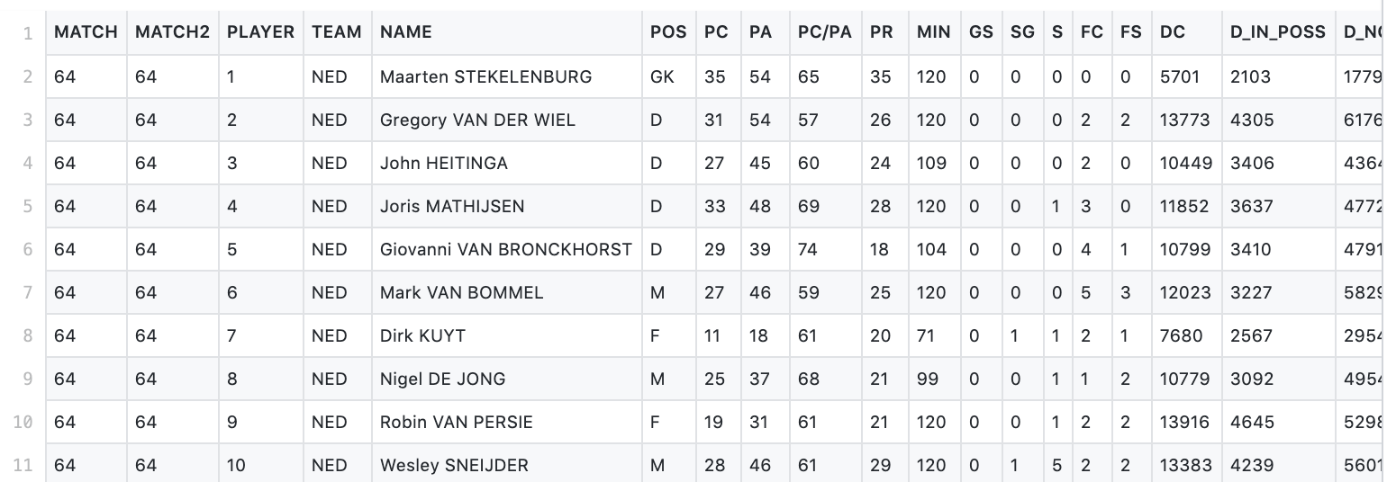
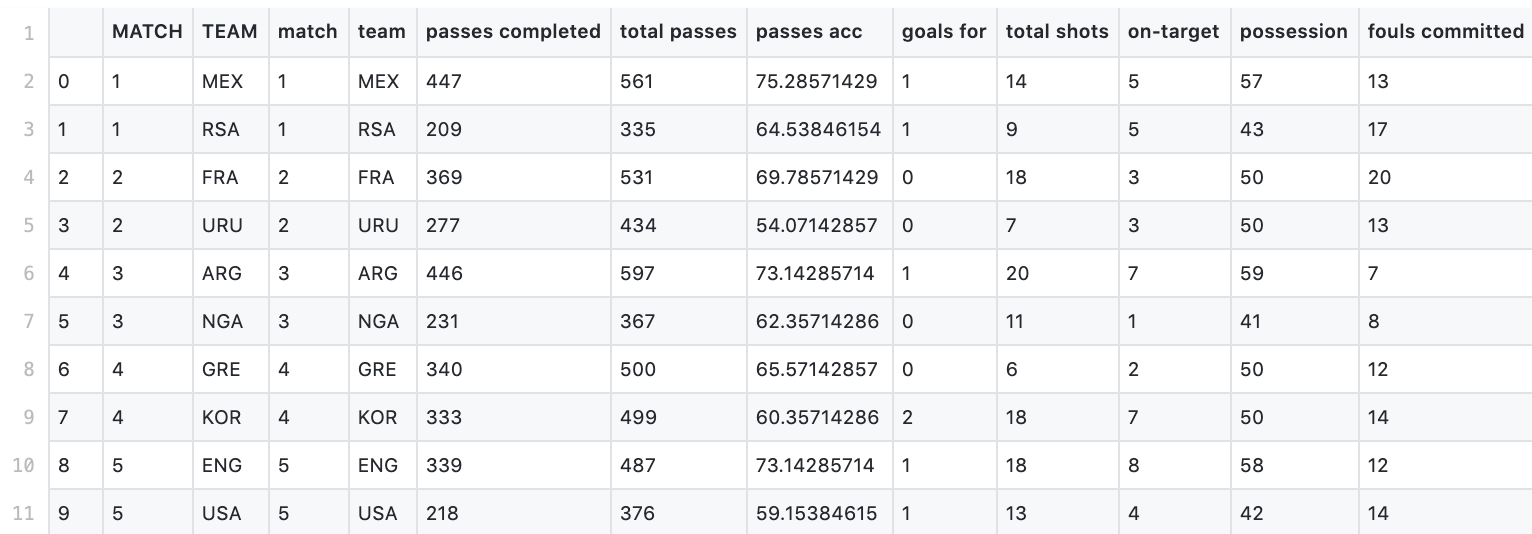
During pre-processing, we cleaned the datasets by aggregating all the player values by teams, so that we no longer had to deal with individual players as our datapoints. We also removed some unnecessary features and included some interesting ones directly from FIFA’s own site. To conclude our pre-processing, we simply combined all three respective datasets into one and added a “year” feature to every datapoint.

This entire process gave us the dataset we used to conduct the rest of our project. To see our processed and cleaned dataset, see clean_combined_data.csv as well as a preview in the image below.

Characteristics and Features

Our final, cleaned dataset consists of 384 datapoints and 22 features. Our features include World Cup Year, Team, Match Number, and all different playing-performance characteristics for each team (IE, passes, possession, fouls committed, etc). Our dataset is arguable temporal, since it originally consisted of three respective datasets that were each corresponding to playing stats during a specific year. However, our final dataset combines these three different years and simply includes the year as one of the features.

Our Approach

We will use a random forest classifier, which randomly selects subsets of features from the dataset and uses gini impurity metric to estimate the likelihood of an incorrect classification of the datapoint under a model trained just on that subset of features. From using this process on several random subsets of features, the model provides the feature’s impurity scores, which we will then use to select the features that greatly correlate to a proper classification of match result.

After identifying the most significant features we will use supervised learning to train a random forest model, as well as serveral other models, to predict the outcome of a match given a certain set of values for each feature.

Why Do We Believe Our Approach Will Solve Our Problem?

We chose a random forest classifier because it performs classification jobs well even on small datasets, scales well with more data, and determines relevant features effectively. Additionally, our solutions are unique in that they combine historial data with our most-important-features analysis to try and predict results.

Data Analysis

Before tackling the machine learning predictions, we did some data analysis to understand trends in our data and deepen our understanding of our dataset.

First, we did a simple feature analysis to see how correlated our features were to match outcome.

We chose to do the same with final position in the tournament.

We also analyzed the FIFA Rank with respect to final position by country. Nations inside the triangular area performed as expected during the World Cup. Nations above and to the left of the triangle performed better than expected, whereas nations below and to the right of the triangle performed worse than expected.

(Note: Final position data for 2018 does not go beyond 16. All teams who did not make it to playoffs are positioned as 17th.)

Experiment

How did we evaluate our approach?

To tackle our problem, we used a multi-headed approach. After preprocessing our data, we conducted several different supervised learning models, ranging from the aforementioned Random Forest to Neural Networks. In the following sections, you will read about our most successful approaches. After setting up the varying different models and appropriately managing our data to allow for the subsequent processing, we chose the top three models in terms of prediction accuracy to dive into more detail.

The results of a game can either be “Win”, “Lose”, or “Draw”. Since we are looking at the FIFA World Cup it is largely in a team’s favor to “Win” rather than “Lose or Draw.” As a result, our classification models have been split into two groups: binary (“Win” and “Not Win”) and ternary (“Win”, “Draw”, or “Lose”) models. We’ve tested our model using Random Forest, Neural Network, Linear Regression, Ridge Regression, SVM, XGBoost Classifier, and an AdaBoost Classifier. We’ve analyzed using cross validation and hyper parametrization while varying data splits and number of features. For some models, we applied Principal Component Analysis, Linear Discriminant Analysis, and Neighborhood Component Analysis, as additions to our classifiers in some cases to improve results. After thoroughly testing various classifiers and applying different parameter combinations, the top 3 based on binary test accuracy were SVM (77.6%), Neural Network (75.0%), and XGBoost Classifier (74.1%). The following sections will review the reasons as to why our proposed model, the Random Forest, was not one of the top 3 classifiers and what made the Neural Network, XGBoost, and SVM more successful. Here’s a summary of our results:

Random Forest

In our initial proposal, we decided to implement a Random Forest in order to train a prediction model. At the beginning of this paper, we explained that we chose a Random Forest because of its ability to perform well with small datasets. The scalability of Random Forests was also important to us. Yet, our Random Forest classifier performed poorly and was not by any means one of our top performers.

What is it?

A Random Forest, or Random Decision Tree, is a kind of classification algorithm. It works, like any decision tree, by continuously splitting a dataset based on some features. Where a Random Forest becomes unique is that it uses a large number of decision trees that work in tandem. The decision trees each come to some prediction, and the prediction that occurred the most times (i.e. had the most votes) is the one that the Random Forest chooses to proceed with. The ability of a Random Forest to perform well is rooted in the large number of decision trees working together, since this inherently helps Random Forests avoid a single tree’s failure when the whole forest is what is ultimately considered.

How did we implement it?

We implemented a 30:70 test to train split on the data. Using the sklearn’s StandardScaler class, we standardized the features by removing the mean and scaling to unit variance. Then using sklearn’s RandomForestClassifier, we did a hyperparameter analysis. We found that the number of estimators were best around 90-120. There was no significant difference between using entropy or gini as the function to measure the quality of a split. An unlimited maximum depth performed best, and since we have a small dataset, computational cost was not a large tradeoff. Through these hyperparameters, we got testing score average of 57.7% for ternary classifciation and 69.3% for binary classification.

Before running our Random Forest classification, we did a feature importance analysis.

We also explored how in-game features (e.g. possession, offsides, sprints, fouls committed, etc.), compared to out-of-game features (e.g. FIFA rank, team value, no. of Players ranked in the top 100) when it comes to classification. To our surprise, out-of-game features were not as successful as we had anticipated. It is comforting to know that money and team prestige cannot buy a World Cup victory. The outcome comes down to the match itself, which is another reason why these games are so hard to predict.

How did it compare?

Now that we understand Random Forests, both generally and in our specific use case, this leaves the key question: why did our Random Forest approach fail? In our case, we can trace the failure to two key problems: lack of data, and the intrinsic difficulty in predicting sports matches. Let’s start with the first issue, a lack of data. Our dataset consisted of only about 300 datapoints. For any sort of machine learning algorithm, this is a tiny amount of data. This made any sort of training, even with a Random Forest that specializes on small datasets, rather difficult. Expanding our dataset further, which we did several times, eventually reached a limit. Finding all the features we needed for past World Cups was not feasible beyond a point due the lack of historic catalogs and data to begin with. The second reason our Random Forest failed is the intrinsic difficulty in predicting a sports match. As Felipe put it, “If there were a good model to predict games with a near perfect accuracy, there’d be no point in playing the games.” The number of variables, measurable and immeasurable, that lead to one team’s victory over another is absolutely expansive. Unfortunately, these two issues coupled together led to the failure of the Random Forest for our World Cup prediction model.

Neural Net

What is is?

Before we look into our first successful model, a Neural Net, let’s try to better understand what Neural Nets are. Neural networks are models inspired by the architecture, function, and layout of the human brain. They work by recognizing patterns in data, even if the data seems to be considerably unrelated. For our case, this was useful because the defining characteristics of what sways a particular soccer match can vary significantly. Neural Nets help us make predictions and classify data even when other algorithms may struggle. They do this by passing an input through hidden layers of neurons that transform the data, to eventually give us an output that is compared to some given goal. The errors the Neural Net made help, in turn, adjust itself so that overtime, it is trained to provide more accurate classifications and predictions.

How did we implement it?

There are a myriad of libraries for implementing Neural Nets, but we chose to keep it simple by using the MLPClassifier class from scikit-learn. This stands for Multi-layer perceptron classifier, which is a fancy name for a Neural Network used for classification. As usual, we set aside 30% for testing and use 70% for training, then standardize the mean and variance.

MLPClassifier has many parameters, including activation function, number of hidden layers, and regularization parameter ⍺. Modifying these three allows us to configure our model without getting lost in a sea of too many hyperparameters. Using a scikit-learn GridSearchCV object for convenience and multithreading support, we can search our hyperparameter space for the values that maximize the cross validation scores.

Initially, we were able to achieve a testing score of 58.6% for ternary classification. The associated hyperparameters were hyperbolic tangent activation function, a single hidden layer with two neurons, and regularization of ⍺=9.8. For binary classification, our neural net surprised us with a testing score of 75.0% for a smaller value of ⍺=5.6. With such a small dataset, we were very happy with these classification results!

Determined to see if we could do better, we seeked guidance from our instructor and TAs, who suggested trying Linear Discriminant Analysis on the dataset before training our models. LDA is a dimensionality reduction procedure which trims a dataset with d features and mlabels down to d’ <= m - 1 features. Since we have 3 labels (“Win”, ”Draw”, ”Lose”), we can use LDA to compress our dataset into either 2 or 1 features. We can also do binary classification with 2 labels (“Win” or “Not Win”), in which case LDA would reduce our dataset to 1 feature.

By performing our analysis again with the LDA-reduced dataset, we managed a slight improvement to a testing score of 63.8%, with the same activation and number of hidden layers, but with a regularization of ⍺=1.1.

However, for binary classification, LDA did not seem to improve our accuracy. We think this is because neural networks strive in larger feature spaces, so training one on a single feature might not yield the best results. Below is a summary of our results.

How did it compare?

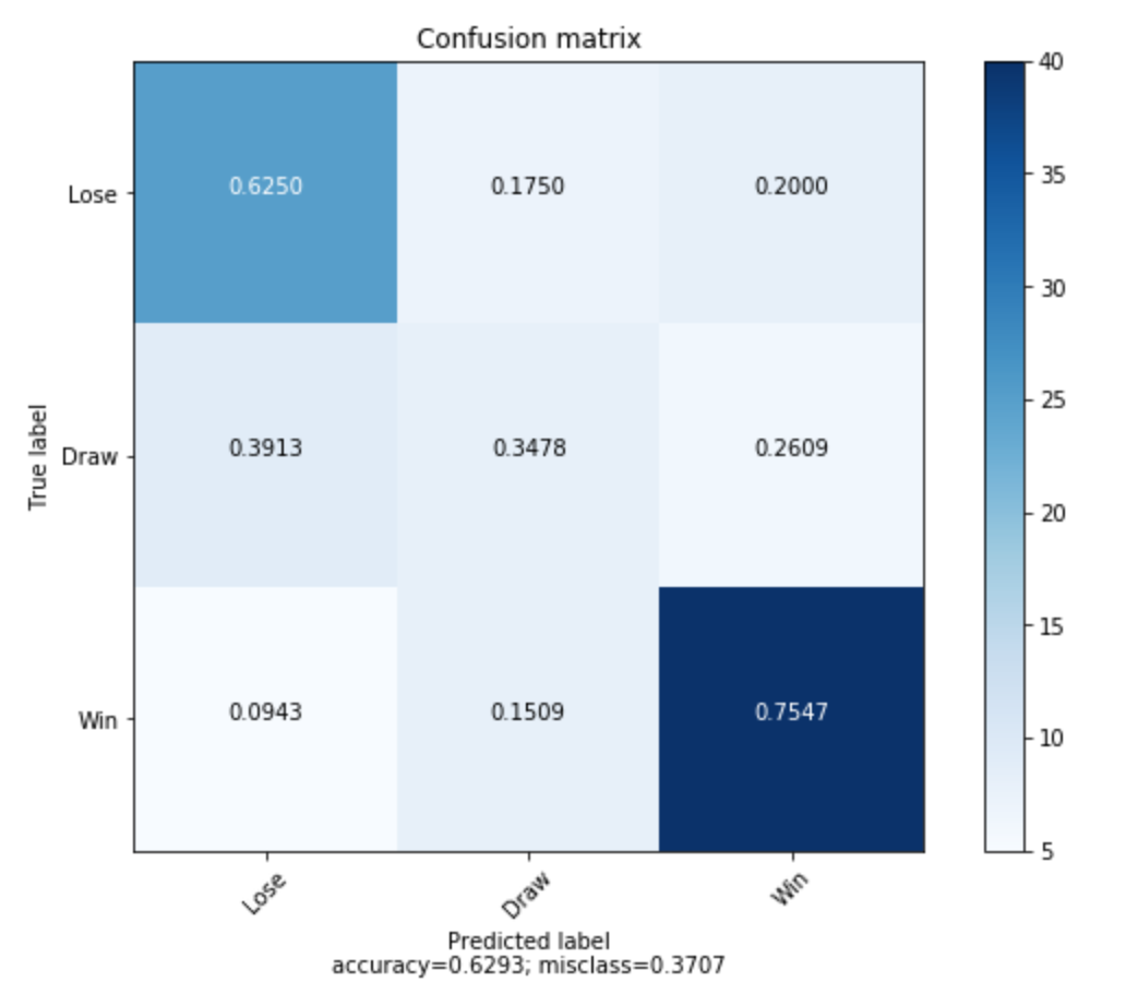
Compared to our performance results with the other classifiers, the Neural Network was consistently one of the best across both ternary and binary classifications. The ternary classification using Neural Networks returned with a test accuracy of 62.9%, while the binary was 75.0%. These results make the Neural Network the second-best performing classifier after SVM. The success of this model can be attributed to the use of the MLP Classifier and finding the optimal hidden layer and value for both classifications. Despite being one of our best models, the Neural Network was limited when applied on to our ternary labels: “Draw”, “Win” or “Lose.” In none of the runs were we able to classify a game either correctly or incorrectly as a “Draw.” This is likely due to our small sized dataset and the limited number of games ending in a “Draw”. There is a smaller number of neural interconnections occurring within our dataset than others. On the other hand, we can see this model’s success in the binary classification where we remove the small “Draw” label and increase the size of another larger label. Overall, the Neural Network was a promising model and one that we are satisfied using to predict our game outcomes.

XGBoost

What is it?

A XGBoost classifier is a meta-estimator that first fits a classifier on the original dataset. It then fits copies of the classifier on the same dataset with adjusted weights so that the subsequent classifiers hone in on more difficult cases to classify.

How did we implement it?

We used the default implementation from Sklearn.ensemble for our predictions. To create the model we first created a pipeline for the games dataset with three steps. Initially the dataset is normalized using a Standard Scaler object from the sklearn preprocessing library. After this step every feature in the dataset has a mean of zero and a standard deviation of one. The second step is to apply the Linear Discriminant Analysis (LDA) on the normalized data, and lastly we fit the data though the XGBoost classifier.

The key parameters of our classifier are the base estimator, number of estimators and learning rate. The base estimator is the model used for the “weak learners” used to cast their votes and make up the “strong classifier” prediction. In this implementation we used decision trees as they yielded the best results. The number of estimators represents the number of weak models to be trained iteratively, which we hyper parametrized to be 50, 75, or 100. Lastly, the learning rate relates to how much the weights for the weak predictions are updated at every iteration. Using a large learning rate (such as ⍺ = 1) leads to big changes every iteration and higher chances of convergence in fewer iterations, however we risk losing the global optimum point for the classifier, therefore we also hyper parametrized alpha to be 0.1, 0.3, 0.5, or 1.

Confusion matrix for ternary classification using XGBoost:

How did it compare?

The best results were obtained for the XGBoost model trained on 100 estimators at a learning rate of 0.1, also using all features. We noticed that increasing the number of estimators or decreasing the learning rate did not correlate to accuracy improvements, so we determined this combination of parameters to be our “optimum solution”. With this model we were able to achieve a 74.1% accuracy during testing for a binary classification (“Win” vs. “Not Win”) and a 62.9% accuracy for testing when applied to a ternary classification (“Win” vs. “Draw” vs. “Lose”), all implementations using a 30:70 test to train split. We found that modifying parameters beyond this point did not lead to improved results. These results puts our XGBoost attempt as the third highest performing model, only behind the SVM and the Neural Net implementations.

SVM

What is it?

A Support Vector Machine (SVM) is an algorithm designed to find a hyperplane or line in an n-dimensional space. They are perfect for supervised learning as they build from the given labels and training results. As a classifier, SVMs are used to separate the various classes of data points. The SVM training algorithm builds a model that assigns new elements to one class or another, making it a non-probabilistic binary linear classifier. This model is particularly impressive, because it takes not linearly separable data in one space and maps it to a higher-dimensional space, making the data now linearly separable. Kernel functions make the mappings possible. There exist many different kernel functions which can be applied during the SVM algorithm to fit the needs of the specific dataset. The algorithm has the objective of creating a plane with the maximum margin between data points of these classes. By maximizing the distance between classes, it becomes far easier to classify an entry as one of the resulting classes.

How did we implement it?

For our support vector machine implementation, we first split our dataset into 30% testing and 70% training. Then, we standardized the features, removing the mean and scaling them all to unit variance. Finally, we used the training data to fit an scikit-learn SVC object (which is an implementation of a support vector machine for classification), observing the 5-fold cross validation scores to determine the the best kernel to use and the best value for the model’s regularization hyperparameterC.

Initially, our analysis determined that a linear kernel with C=1.1 was the best, yielding a testing score of 59.5%. We can then apply LDA to reduce our dataset to two features.

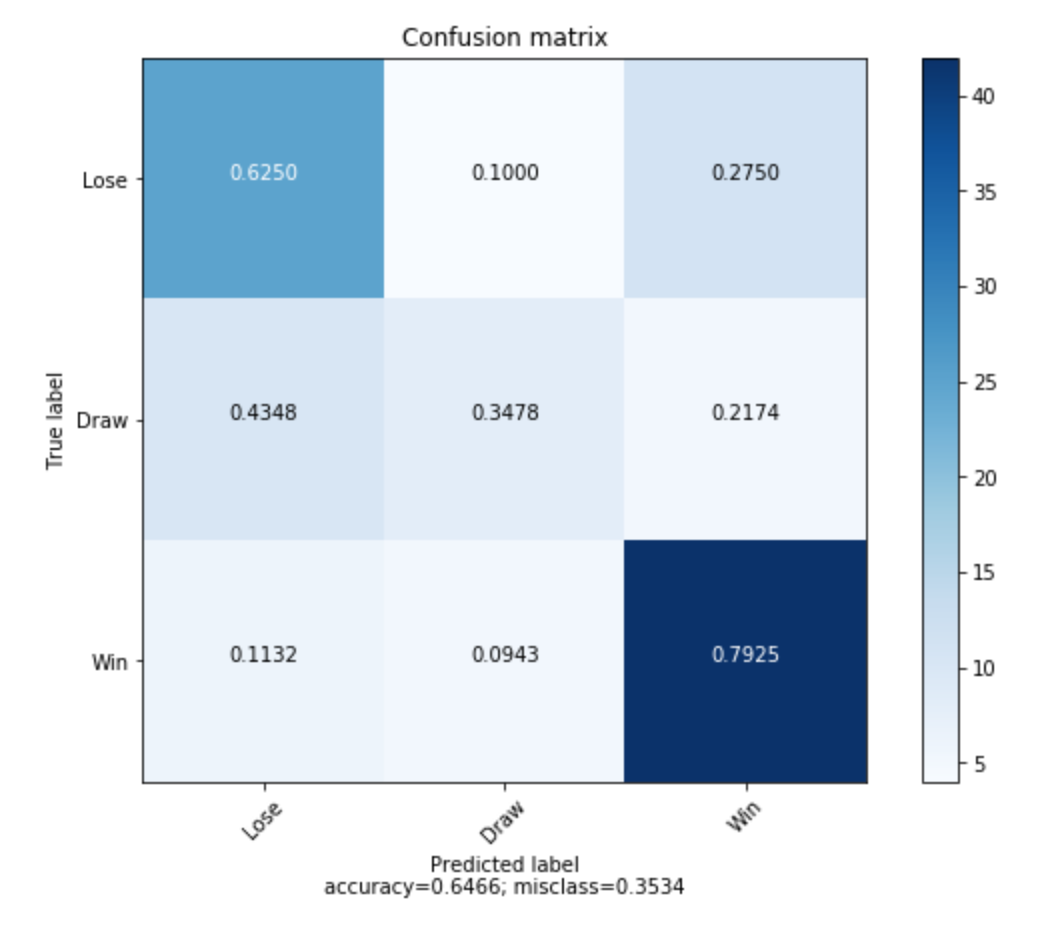
Performing the same analysis as before on both of these reduced datasets, our new best hyperparameters for ternary classification were a radial basis function kernel with C=0.55, which yield a testing score of 64.6%! This is a 5% improvement, by using 2 features instead of 22!

Confusion matrix for ternary classification using SVM with LDA:

An added bonus is that with a 2 feature space, we can visualize our model’s decision boundaries and performance with these best case hyperparameters:

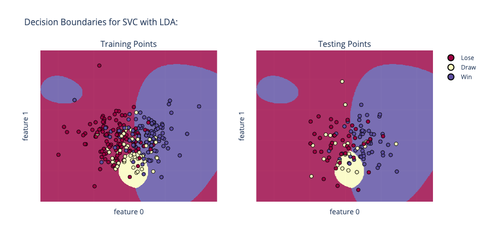
The round shape of the model’s learned decision boundaries are due to the radial basis function kernel. On the other hand, a linear kernel would cause the decision boundaries to be straight lines.

Now, for binary classification, LDA will always compress the dataset into one feature. Performing a similar cross validation analysis on this single feature dataset, we found that the best hyperparameters for deciding between “Win” and “Not Win” were a linear kernel with C=0.45, which yields a testing accuracy of 75.0%! It’s incredible that we can achieve this accuracy by looking at a single feature! These binary classification results are on par with our Neural Net’s performance.

How did it compare?

Of all the classifiers applied to our model, SVM ranks the best in both binary and ternary classification. This is due to the pairing of LDA and our linear kernel with our SVM. Traditionally a large number of features is greatly advantageous to the optimization of SVM classification, but in this case, we have been able to reduce our features down to one highly linear feature. Applying LDA to our feature set has allotted us with one very linear feature which has made the linear kernel SVM classification very simple. As a result, this has been our best model at predicting the result of a FIFA World Cup soccer game.

Conclusion

As we reach the end of our project, it is important to take a look at where we started. Our initial proposal, drafted months ago, stated that we would train a model using the Random Forest classifier to predict World Cup matches given data from the past three World Cups. In reality, we trained several different types of classifiers, all with varying results. But more paramount than our proposal is our goal: can we successfully train a model to predict World Cup matches? With all the models we trained, our highest accuracy achieved was 77.6% for binary classifciation and 64.6% for ternary classification. Although not perfect, it is a much better predictor than a random guess which would be around 50% and 33% respectively. Given the nature of these games as being inherently difficult to predict, as well as the fact that this was our first foray into machine learning, we would say that our predictions are a success!

References

Bunker, Rory P., and Fadi Thabtah. “A Machine Learning Framework for Sport Result Prediction.” Applied Computing and Informatics, vol. 15, no. 1, Jan. 2019, pp. 27–33., doi:10.1016/j.aci.2017.09.005.

Kapadia, Kumash, et al. “Sport Analytics for Cricket Game Results Using Machine Learning: An Experimental Study.” Applied Computing and Informatics, 21 Nov. 2019, doi:10.1016/j.aci.2019.11.006.

Mccabe, Alan, and Jarrod Trevathan. “Artificial Intelligence in Sports Prediction.” Fifth International Conference on Information Technology: New Generations (Itng 2008), 18 Apr. 2008, pp. 1194-1197., doi:10.1109/itng.2008.203.

Ulmer, Ben, Matthew Fernandez, and Michael Peterson. “Predicting soccer match results in the English Premier League.” PhD diss., Ph. D. thesis, Doctoral dissertation, Ph. D. dissertation, Stanford, 2013.